Part 2 (Theory): The Monte Carlo Simulation

Introduction

As discussed in previous chapters, we need to simulate light photon beams in order to determine the true color of our surface.

The “Monte Carlo” simulation provides a method to do this. The name “Monte Carlo” derives from the randomness used in the method; we use random values at several stages and also use a Russian Roulette approach to ‘killing’ the photon beam.

The general approach is to create a beam of light at a position (i.e. the origin, (0,0,0)), give it a direction and wavelength. We then iterate for n times, each time moving the photon beam further into the material, scattering, absorbing and reflecting as it goes. We run the simulation for each wavelength of light we care about – i.e. 380nm-780nm, at 10nm intervals.

We store the information we want to keep (in our case, the reflectance) in “bins” that we add to at each iteration stage.

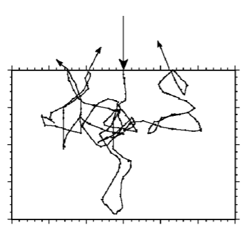
Here’s the general flow for Monte Carlo simulation:

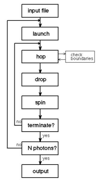
To translate this: We launch a photon with a weight (w = 1.0), we move the photon (hop) and check if we have changed boundaries between tissues. At the drop stage we interact with the tissue (absorption, etc). Next, we redirect the photon based on scattering (spin), and finally we run a simple roulette to see if the photon should terminate. If we don’t terminate, we keep moving the photon. If it does terminate, we launch the next photon. This process continues until we run out of photons (N photons).

We will now cover each of these steps more deeply:

Launch

To launch we need three things:
1. A starting location
2. A starting direction to hop
3. A “weight”

The first two should be fairly explanatory. We start at (0,0,0) and initially move forwards – we will use +z as our forward axis into the tissue.

We will use an “isotropic point source” to launch our photon. This simply means we have no preferred direction. Our starting position shall be:

x = 0, y = 0, z = 0

And our launching trajectory will be:

RND = 0.0 <= n < 1.0
cosθ = 2 RND – 1
sinθ = √(1-cosθ)
ϕ = 2 π RND
if ( ϕ < π )
 sinϕ = √(1-cos²ϕ)
else
 sinϕ = –√(1-cos²ϕ)

ux = sinθ cosϕ
uy = sinθ sinϕ
uz = abs(cosθ)

The weight, w, is what we shall use to track how much of the photon’s energy is remaining. In our simulation we shall define a zone around the origin through which we will collect any photons that head back into it. By summing the weight of these photons, at all the wavelengths of light we are sampling, we will end up with our reflectance values.

Hop

Hop consists of two parts: A Boundary Check and Moving. In our two-layer model, we have an upper epidermis, a lower dermis layer and the external medium – air.

For our purposes, we count anything above the epidermis as ‘escaped’, and if it is close enough to the beam source (the launch position), we capture its weight.

We’ll start by calculating our new position, this is calculated by:

µ_t = µ_a + µ_s
where µ_a is the absorption coefficient, and µ_s is our scattering coefficient

s = -ln(RND)/µ_t
x = x + s ux
y = y + s uy
z = z + s uz

Now we check whether it has escaped the tissue by checking if the uz property is < 0.0. However, the photon may partially reflect back into the tissue at the boundary, due to total internal reflection.

How do we calculate this?

First, let’s start by moving the photon back to the point where it left the tissue, and move it just back to the surface. We calculate the partial step, s₁:

s₁ = abs(z/uz)

Then, retract the full step:

x = x – s ux
y = y – s uy
z = z – s uz

and then add in the partial step, back to the boundary:

x = x + s₁ ux
y = y + s₁ uy
z = z + s₁ uz

Now our photon is at the surface, we use the Fresnel equation to determine how much of the energy was reflected back into the tissue:

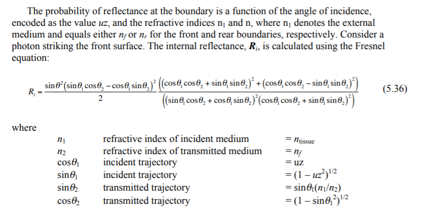
We can now calculate the weight that has escaped the tissue with:

R_e = 1 – R_i

This can then be stored in our ‘bin’

r = √(x² + y²)
ir = r/dr
reflectionBin[ir] = R_e

where dr is our radial bin size, (radial size of our photons/number of bins). I have glossed over these parameters, as its a bit deep for this tutorial. Simply put, r is the radial position of the photon, dr gives us a ‘depth’. Although we simulate the Monte Carlo simulation in 3D Cartesian coordinates, we actually only care about getting data for radial position and depth, as the photon beam is cylindrical.

Finally, we bounce the photon back into the tissue, with it’s escapes weighting removed:

w = R_i * w
uz = -uz
x = (s-s₁) * ux
y = (s-s₁) * uy
z = (s-s₁) * uz

Drop

Our drop stage is the easiest. As we have calculated the reflectance of the tissue above, we simply need to decrement the weight of our photon by the amount absorbed by the surface albedo.

Which albedo value we use depends on the layer in the skin we are in:

if z <= epidermis_thickness
 albedo = σ^epidermis_s/(σ^epidermis_s + σ^epidermis_a)
else
 albedo = σ^dermis_s/(σ^dermis_s + σ^dermis_a)

Now to reduce the weight:

absorb = w * (1 – albedo)
w = w – absorb

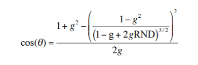
Spin

Next up: scatter the photon! We need two angles of scatter, θ (deflection) and ϕ (azimuthal). The source paper goes into great detail as to why we use the following formula (the HG function) to calculate θ, if you want more information, but for the purposes of this tutorial, we’ll just describe it:

The azimuthal angle is a bit less verbose:

ϕ = 2π RND

Now we can calculate the new angles, we need to update our photon trajectories:

if (1 – abs(uz) <= 1 – cos0) : # close to perpendicular.
 uxx = sinθ * cosϕ
 uyy = sinθ * sinϕ
 uzz = cosθ * SIGN(uz)
else:
 temp = √(1.0 – uz * uz)
 uxx = sinθ * (ux * uz * cosϕ – uy * sinϕ) / temp + ux * cosθ
 uyy = sinθ * (uy * uz * cosϕ + ux * sinϕ) / temp + uy * cosθ
 uzz = -sinθ * cosϕ * temp + uz * cosθ

ux = uxx
uy = uyy
uz = uzz

Where SIGN(x) is x >= 0 ? 1 : 0

Terminate

The photon will continue to propagate naturally and will never terminate naturally (w will simply get smaller). We therefore need a way to terminate the photon.

This is done by simply creating a random number and comparing it to the remaining energy of the photon, if the photon weight is below a threshold:

if w < THRESHOLD
 if RND > CHANCE
  terminate the photon

However, this will not conserve energy as we are removing [the leftover] energy from the simulation (and energy cannot be destroyed). We therefore need to conserve the energy.

We do this by adding energy into photons that are not terminated by the random chance, i.e., if we expect that 9/10 photons will terminate with the random check, we multiply the energy by 10-fold on the one photon that did not terminate and allow it to continue. This maintains energy conservation laws. Therefore, the actual implementation is as follows:

if w < THRESHOLD
 if RND > CHANCE
  terminate the photon
 else
  w = w/CHANCE

Extracting The Reflectance

The final step in the simulation, after letting it run through as many iterations as we want, is to get the data back out.

To do this, we simply iterate over the ‘bins’ we added weights into earlier, summing up their weights, and diving it down by the number of photons we used in our simulation:

for i = 0; i < length(reflectionBin); i++
 R_t = R_t + reflectionBin[i] /Nphotons

Where R_t is total reflection

Now we do this for each wavelength we want to sample, and we will get a nice set of data describing the reflection at each of those points. We’ll implement this all in Python in the next part.