Getting Going First things, open Python IDLE 3.8 (64-bit)… and create a new file… Save this file as Skin_Reflectance_Generation.py, or similar. Skin_Reflectance_Generation.py If you have a preferred IDE for authoring Python, feel free to use that. I wanted to keep this tutorial minimal, hence I’m using IDLE. Chromophores and Power Curves We now need to convert all those formulae on the previous chapter into Python code. Let us begin by first creating a class and instancing that class. This is just the boiler-plate code to get us going: class SkinAbsorption: def __init__(self): print(“init SkinAbsorption”) Running this code should result in: Now we need to generate the absorption coefficients. In order to go through each wavelength, we’ll need a for loop. We’ll put this into a new function, in our class like so: We don’t need a value for every nm of light wavelength, 10nm intervals will suffice. We get enough precision without the overhead of hundreds of values. Running this code will output every wavelength we’re going to calculate values for. In order to calculate values, we need to pass in values for our melanin fraction (Cm), hemoglobin fraction (Ch) and melanin blend (βm). Jimenez et al [2010] helpfully provide us with suitable ranges for us: Its also worth noting that Jimenez et al [2010] also state we should sample cubicly to maximize texture space usage, so our sampling values should be:Cm = [0.002, 0.0135, 0.0425, 0.1, 0.185, 0.32, 0.5]Ch = [0.003, 0.02, 0.07, 0.16, 0.32]Our blend value does not need to be cubic, we’ll do 3 samples to keep it fast and interpolate the values in our shader later.βm = [0.01, 0.5, 0.99] We’ll extract some more for loops in functions from these, like so: At the moment, running our code will just dump a list of wavelengths and our fractional and blend values, like so: Now for the math!We’ll replace our print line (on Line 21) with the following in order to generate our coefficients for epidermal absorption and scattering: Running those code should produce a lot of values! We don’t have to make sense of these yet, we’ll debug these later. Extracting Graph Data to CSV The dermis is a bit more complicated as we can’t easily reconstruct the data. What we need to do is to get actual data that maps wavelengths to coefficients. There is a file format, known as CSV, which stands for “comma separated values”. It is simply a list of rows and column values, with each column separated by a comma and each row in on a new line. Its structure looks identical to the values we just printed in the image above, i.e.: columnName1,columnName2,columnName3 234,456,789 136,234,567 … You can upload an image, define the graph boundaries and axis, and get out CSV values as a file. It is perfect for this sort of thing. Let’s graph a graph that has the data we want to sample, and load it into graphreader: Make the blue box surround the values from 300-800 (we can remove rows we don’t want after). Then start double clicking add to add points along one of the lines. Be sure to set the axis appropriately: Then, “Redraw fix-points”, then “Generate curve”, you will get the following values output: These values are measured in [cm-1M-1], so we need to divide these down by 100.My CSV files for oxygenated and deoxygenated hemoglobin are here. Feel free to download them if you have issues with graph reader.Save them into the same location as your python file as O2hb.csv and hb.csv respectively: Now we can update our dermis absorption section, add this to our code between epidermis and the scattering calculation: This won’t work yet! We need to load our CSV data. Above the __init__ function add the following: class SkinAbsorption: O2Hb = {} Hb = {} def __init__(self): #… Then, in the __init__ function, do the following: This will open and read the CSV files and write them to a python dictionary, where each key-value pair is:{ key : value} = { wavelength : absorption coefficient }In other words:{ 380 : 97.58 , 390 : 100.024, …} Running it, you should get this sort of garbage in your console window! Debugging Values to CSV The final thing to do is to check all our values are as we expect. As you can see, we’re dumping a load of values to the console that look remarkably like CSV values already – this is no coincidence. Instead of printing the values, we shall compress them into a string and write this out to a CSV ourselves, so we can create the debug graphs we want in Excel (or other Spreadsheet software). First, lets remove the printing and convert it to an appended string. We’ll set the first line to be our column headings, and make sure we add the wavelength of light for easier reading later. Like so: This will now output a CSV in our folder: For completeness, here is the Python code so far: class SkinAbsorption: O2Hb = {} Hb = {} def __init__(self): print(“init SkinAbsorption”) HbFile = open(‘hb.csv’, “r”) O2HbFile = open(‘O2Hb.csv’, “r”) HbLines = HbFile.readlines() for line in HbLines: splitLine = line.split(“,”) self.Hb[int(splitLine[0])] = float(splitLine[1].rstrip(“\n”)) O2HbLines = O2HbFile.readlines() for line in O2HbLines: splitLine = line.split(“,”) self.O2Hb[int(splitLine[0])] = float(splitLine[1].rstrip(“\n”)) HbFile.close() O2HbFile.close() def Generate(self): CSV_Out = “Wavelength,Eumelanin,Pheomelanin,Baseline,Epidermis,ScatteringEpi,ScatteringDerm,Dermis\n” groupByBlend = [] for Bm in [0.01,0.5,0.99]: groupByMelanin = [] for Cm in [0.002,0.0135,0.0425,0.1,0.185,0.32,0.5]: groupByHemoglobin = [] for Ch in [0.003,0.02,0.07,0.16,0.32]: values = self.GetReflectanceValues( Cm, Ch, Bm ) CSV_Out = CSV_Out + values groupByHemoglobin.append(values) groupByMelanin.append(groupByHemoglobin) groupByBlend.append(groupByMelanin) CSV_Out_File = open(“AbsorptionValues.csv”,”w+”) CSV_Out_File.write(CSV_Out) CSV_Out_File.close() return groupByBlend def GetReflectanceValues(self, Cm, Ch, Bm): CSV_Out = “” wavelengths = range(380,790,10) for nm in wavelengths: # First layer absorption – Epidermis SAV_eumelanin_L = 6.6 * pow(10,10) * pow(nm,-3.33) SAV_pheomelanin_L = 2.9 * pow(10,14) * pow(nm,-4.75) epidermal_hemoglobin_fraction = Ch * 0.25 # baseline – used in both layers baselineSkinAbsorption_L = 0.0244 + 8.54 * pow(10,-(nm-220)/123) # Epidermis Absorption Coefficient: epidermis = Cm * ((Bm * SAV_eumelanin_L) +((1 – Bm ) *
Part 1 (Theory): What Makes Skin Color?
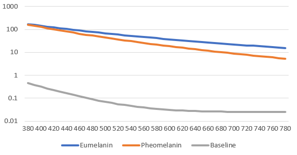
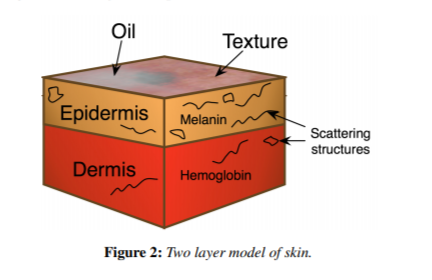
Chromophores A chromophore is the part of any molecule that gives that molecule its color. It gives color by absorbing different wavelengths of light and reflecting others. An examples of a chromophore you may be familiar with is chlorophyll. It exists inside plants, reflecting green light, to give the plant its green-colored leaves. It absorbs the other colors of light to create energy through the process of photosynthesis. Such chromophores also exist in your skin. The one you are probably most familiar with is melanin, which creates darker skin in higher concentrations. In the skin, melanin comes in two types: eumelnain and pheomelanin. Eumelanin is the most abundant of the two types, and is largely responsible for making skin darker, giving it a more brown or black tone. Pheomelanin causes a reddening of the skin and is found in lower concentrations. An interesting thing to note is that skin can have differing ratios of these types. The blend of these two chromophores is what tends to give us the variance in black skin in different ethnicities, such as across Africa and the Middle East. There is one more chromophore that greatly affects skin color: hemoglobin. This is responsible for the redness of skin. It is the reason that shining a bright light through a fingertip causes the fingertip to look red. It is what causes blushing. Hemoglobin has a significant impact on final skin tone, and especially with lighter skin colors, as less red light gets absorbed by the melanin. Going forward, we’ll occasionally refer to each of these chromophores with the following notation (particularly in formulae): Cm = “Melanin Fraction”, or, “the amount of melanin in the skin” βm = “Melanin Blend”, or, “what is the proportion of emuelanin to phemelanin?” Ch = “Hemoglobin Fraction”, or, “the amount of hemoglobin in the skin” We will sometimes further split the hemoglobin fraction up, as there is differing levels of hemoglobin in different layers of the skin. Che refers to the hemoglobin fraction in the epidermis, Chd is for the dermis. More on this later! Absorption, Reflection, Scattering We can’t proceed any further without a solid understanding on what makes color, more generally. The human sees visible wavelengths of light. These wavelengths range from approximate 380nm to 780nm: Figure 2: Wavelength of the visible spectrum is at the top, on the x-axis. We tend to categorize light into boxes, such as “red”, “yellow”, “green”, etc., but this is not strictly correct. These categorizations are crafted by humans to broadly describe the colour of an object, but they don’t work when we want to describe what is actually happening to the light. If an object appears red, that is because it absorbs all, or most, of the wavelengths of light outside of the red wavelengths (<570nm), and reflects the red values back away and into our eyes. We can therefore describe a color in a more factual way by plotting which wavelengths it absorbs. We can visualize this as a graph. Here is such as graph for two types of chlorophyll: We know that chlorophyll is green, and the graph supports this. We can see that it absorbs blue and red values, leaving green wavelengths reflected towards our eyes. The problem we have is that this absorption graph is not telling us how much green gets reflected back into our eyes. This is because the green wavelengths may bounce back out the tissue, or simply pass straight through it. It is this reflected information that gives us the color of the object, so we need to be able to calculate it. To figure out how to get the reflectance values, we need to understand exactly how light behaves inside an object such as a chloroplast or in the skin. As a light photon hits a chromophore, if the wavelength is absorbed by the chromophore, the photon ‘dies’ (as far as we are concerned). If it is not absorbed it is reflected back out. The complexity arises in that the photons hit things within the structure of the medium it is travelling. It causes the photons to bounce and scatter. As they do so, they lose energy. Others may reflect back out the medium, but in a direction that never reaches our eyes. We therefore need to model this behavior programatically in order to obtain correct reflectance values. The Structure of Skin Before we can start getting into simulating this phenomenon, we need to look at the physical structure of the skin. The skin has two primary layers (at least as far as we care about for skin color): the epidermis and the dermis. The epidermis is the upper layers of skin and predominantly contain our melanin. The dermis refers to the remaining skin below this depth and mainly contributes color through hemoglobin. Figure 5 (Donner et al. [2008]) The dermis also has slight absorption from what we call the “baseline”. This is essentially “everything else that isn’t hemoglobin”. Handily, Donner et al. [2008] provides an illustration for this baseline and other chromophores: Figure 6 (Donner et al. [2008]) We have quite a few factors contributing to absorption, we now need to get this graph data itself (so we can use it in our simulation) and we need to factor in skin layers. The Math Donner et al [2008] helpfully provide how they calculated their absorption and scattering coefficients that they used in their model to generate skin tones Melanin As you can see in the graph above, both melanin types have a fairly smooth curve. These are easy to generate by using a simple power curve. σema(λ) = 6.6 x 10¹⁰ x λ-3.33 mm-1 Where σema is the eumelanin absorption coefficient, σpma is the pheomelanin absorption coefficient and λ is the wavelength of light If this is the first time reading this sort of notation, the way we use these numbers is to replace “λ” with a wavelength. For example, to calculate the eumelanin absorption coefficient for 400nm we

Introduction: Setting Up
Getting Python We’re going to use Python for our producing out LUT. The code can be written in any language, if you prefer. Python was just my preference for prototyping the initial work with, and I stuck with it. You’ll need a version of Python that is 3.0 or higher. This was all written in Python 3.8, so if you wish to avoid potential issues from incompatilbities, use that version. The other important thing is that you need to install and run the 64-bit version. Monte Carlo simulations benefit from the precision, as we can deal with incredibly small numbers. Make sure when installing it, that you add python to your PATH variable. All this does is enable you to call “python” in the command line from any directory on your PC. Getting Packages The next thing we need to do is grab a Python package. We’ll discuss later what we use this particular package for, but for now, let’s just make sure we’ve got it ready. Open a command line by pressing the Start icon and searching for “cmd” Then type the following and press return: python -m pip install –upgrade Pillow Like this! This command runs the pip program that came bundled with Python. It is a package manager and will install the Pillow package. Pillow is a package we will use to generate out LUT image file later. Getting Unreal Engine 4 Next, get yourself a copy of Unreal Engine 4. You need to head to: You will need to get the Epic Games Launcher from there – you will also need an Epic Games account if you don’t have one. Once you have Epic Games Launcher, open it up. Head to “Unreal Engine” on the left navigation pane, click the Library tab and add a new Engine Version if you need one. You can read the full installation docs here if you have an issue: I used 4.25.1 for this tutorial. If you want to use the same version, grab that. We’ll get the correct project files later, in Part 4. Just want the finished projects? If you just want the complete, finished project files you can find that here: <missing link – will re-up!> Ready to continue?
Physically Modeling Skin Tones
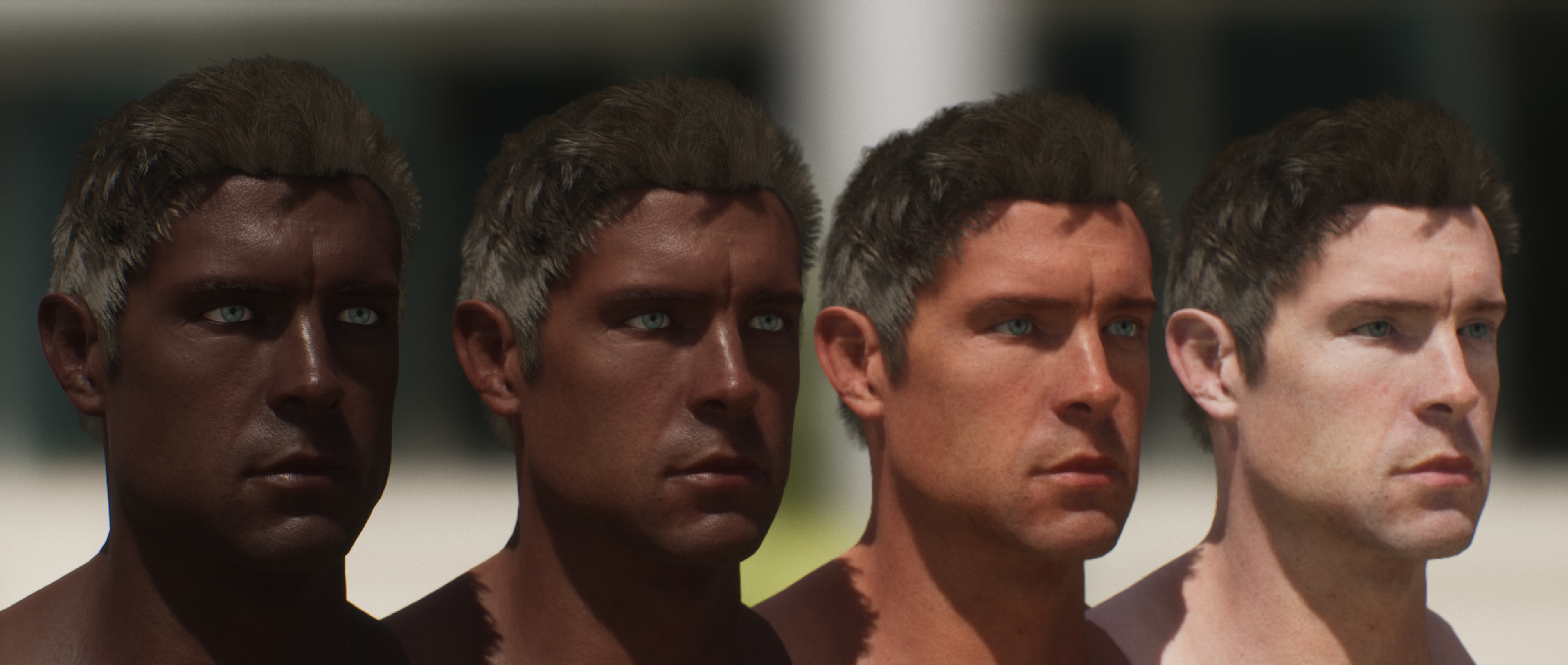
https://half4.xyz/wp-content/uploads/2020/08/Project.mp4 Some of the types of effects you can achieve In this tutorial series, we will cover a novel approach to coloring skin tones in realtime. Our technique will: Generate physically correct skin tones based on Monte Carlo reflectance simulations from spectral absorption data. Enable the realtime changing of skin color, whilst maintaining underlying pigmentation (such as blemishes, scars, moles, pink lips, even make-up) Support tan lines and realtime blushing Generate physically correct skin tones based on Monte Carlo reflectance simulations from spectral absorption data. Why Do This? Motivations for this approach. More Diversity For Less Work Achieving ethnic diversity in games is an important goal, and one that is so critically undervalued and ignored. This technique will allow to pick from a wide range of skin colors, and change the skin color of our characters, without having to re-author textures, or have convoluted workflows that normalize textures (i.e. greyscale textures) to hack a result. There is no reason not to even randomize your skin tones with this approach and get a truly diverse cast of characters. More Believable Characters “Facial appearance depends on both the physical and physiological state of the skin. As people move, talk, undergo stress, and change expression, skin appearance is in constant flux. One of the key indicators of these changes is the color of skin. Skin color is determined by scattering and absorption of light within the skin layers, caused mostly by concentrations of two chromophores, melanin and hemoglobin.“ Jimenez et al. [2010] To get more convincing skin color, we need to be able to change the color of the skin at run time, such as with blushing, or when angry. We need to be able to “redden” the face. In addition, we want our skin color to be physically-based. That is, we won’t want to pick from edited photos to sample our skin color – we want an albedo that is grounded in real values of human skin pigmentation. This way, we won’t need to spend as long calibrating our ‘guessed’ skin tones against real world photos – we will just have real values to select from. Learn About Spectral Values and Monte Carlo Simulation There’s no better excuse to learn something than for the sake of it! This will hopefully teach you something new. I had to learn many of the techniques demonstrated here just for this tutorial because I couldn’t find tutorials covering much of it anyway. Hopefully I can share these learnings, because Spectral Aborption, reflection and Monte Carlo simulations are great to have in your toolbox. Table of Contents Physically Modeling Skin Tones Introduction: Setting Up Part 1 (Theory): What Makes Skin Color? Part 1 (Practical): What Makes Skin Color? Part 2 (Theory): The Monte Carlo Simulation Part 2 (Practical): The Monte Carlo Simulation Part 3 (Theory): Spectral Reflection & Color Spaces Part 3 (Practical): Spectral Reflection & Color Spaces Part 3b (Practical): Python Imaging Library (Pillow) Part 4: Skin Shader Part 5: Extending the Shader Part 6: Concluding Notes