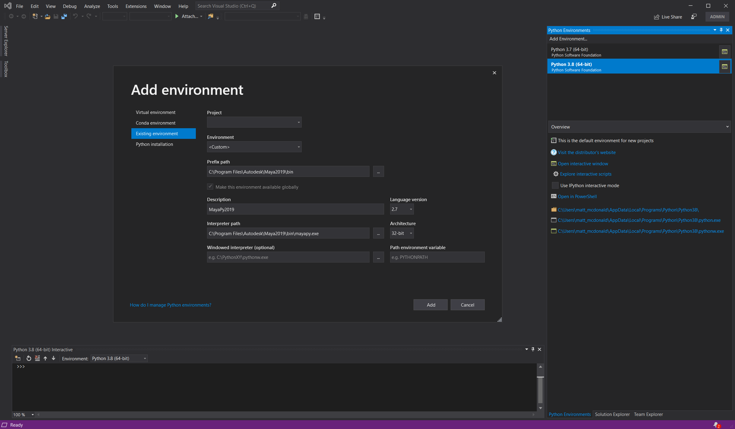
[I’m improving this page, WIP] There are plenty of ways to get up to speed with an IDE for developing Maya tools & plugins. Anecdotally, I’ve found not many studios enforce a particular IDE for Maya development, so this is how I’ve usually got mine configured. Prerequisites An IDE – I use Visual Studio, but VS Code & Eclipse work fine. Getting Started Once you’ve installed those tools, locate where you installed Qt to, and find this application: ~\Qt\Qt5.6.1\5.6\mingw49_32\bin\designer.exe Put a shortcut to this on your Desktop (or wherever). You can run this to build Maya-compatible .UI files Next, run Maya and run this command in Python: import maya.cmds as cmds cmds.commandPort(name=”:7001″, sourceType=”mel”) cmds.commandPort(name=”:7002″, sourceType=”python”) You can, if you wish, add this to you userSetup.py/userSetup.mel file in your Maya scripts path. I also head into VS and add in the Maya Python paths, so you get all the Maya-specific PyMEL commands. You can do this by adding Maya’s python interpreters to a new environment: Open up Designer and make yourself a basic UI, like so: Save this as “MyCustomUiFile.ui” in: C:\Users\<username>\Documents\Maya\<maya version, i,e, ‘2019’>\scripts\ Now, you can use the following termplate to open the UI and hook up events: import os import sys import site from PySide2.QtCore import SIGNAL try: from PySide2.QtCore import * from PySide2.QtGui import * from PySide2.QtWidgets import * from PySide2 import __version__ from shiboken2 import wrapInstance except ImportError: from PySide.QtCore import * from PySide.QtGui import * from PySide import __version__ from shiboken import wrapInstance from maya import OpenMayaUI as omui from PySide2.QtUiTools import * from pymel.all import * import maya import maya.cmds as cmds import pymel.core as pm import pymel.mayautils as mutil mayaMainWindowPtr = omui.MQtUtil.mainWindow() mayaMainWindow = wrapInstance(long(mayaMainWindowPtr), QWidget) windowId = “MyCustomUI” USERNAME = os.getenv(‘USERNAME’) def loadUiWidget(uifilename, parent=None): “””Properly Loads and returns UI files – by BarryPye on stackOverflow””” loader = QUiLoader() uifile = QFile(uifilename) uifile.open(QFile.ReadOnly) ui = loader.load(uifile, parent) uifile.close() return ui class createMyCustomUI(QMainWindow): uiPath = “C:\\Users\\” + USERNAME + “\\Documents\\maya\\2019\\scripts\\MyCustomScript\\UI\\MyCustomUiFile.ui” def onExitCode(self): print(“DEBUG: UI Closed!\n”) def __init__(self): print(“Opening UI at ” + self.uiPath) mainUI = self.uiPath MayaMain = wrapInstance(long(omui.MQtUtil.mainWindow()), QWidget) super(createMyCustomUI, self).__init__(MayaMain) # main window load / settings self.MainWindowUI = loadUiWidget(mainUI, MayaMain) self.MainWindowUI.setAttribute(Qt.WA_DeleteOnClose, True) self.MainWindowUI.destroyed.connect(self.onExitCode) self.MainWindowUI.show() # You can use code like below to implement functions on the UI itself: #self.MainWindowUI.buttonBox.accepted.connect(self.doOk) #def doOk(self): #print(“Ok Button Pressed”) if not (cmds.window(windowId, exists=True)): createMyCustomUI() else: sys.stdout.write(“tool is already open!\n”) That should at least get you going with a basic interface to work from.

Quick Tip: Sort Translucency (UE4)
If you’ve ever made translucent objects in Unreal Engine, or Unity (or just about any modern 3D engine), you’ll have possibly encountered this issue, where parts of your mesh render incorrectly infront or behind of itself. Why does this happen? The UE4 renderer will render all opaque objects to the various GBuffers first. When rendering opaque objects, UE4 writes to a Depth Buffer. The Depth Buffer stores depth information for each pixel (literally “depth from the camera” – a Depth Buffer value of 100 is 100 units from the camera). When rendering a new opaque object we can test the pixel’s depth against this buffer. If the pixel is closer, we draw that pixel and update the Depth Buffer, if it further away (i.e. “behind and existing pixel”), we discard it. Conveniently explained here by Udacity After rendering opaque objects, it then moves on to Translucent objects. The renderer works in a similar way – taking each object and rendering them, checking against the depth values already rendered by the opaque pass. This works fine for simple things such as windows, where you wont get a mesh with faces infront/behind. However, it breaks down under these circumstances. This is because when given a mesh, the renderer tackles the faces by their index. This means it renders the triangle that uses vertices {0,1,2} first, then continues up the chain. This means it may render faces in an order that does not match the order they are in front of the camera. This means some faces are rendered in the wrong order. When rendering opaque objects, this isn’t a problem as every pixel it either fully occluded or not occluded – with Translucent objects, this isn’t the case and we get pixels that stack. This is the same mesh, but with different vertex orders. Note the different pattern of overlaid faces. The CustomDepth buffer works identically to the Depth Buffer, aside from the fact that it only renders objects into the buffer that you define – including Translucent ones. By using this buffer and doing a simple check in our material, we can make pixels that are located behind other pixels in our mesh fully transparent, making them disappear. One caveat: You will not see any parts of the mesh behind itself. I.e., if your mesh was made of two spheres, with one inside the other, you would not see the internal sphere rendered at all. Its a trade-off. There are other solutions to this problem, but this is the simplest and works in most cases. On the left we have the default Translucency. On the right we have sorted Translucency. As you can see, we can no longer see back faces – this may not be what you want. Rendering to the CustomDepth Bufffer Step 1 is to get your mesh and locate the “Render CustomDepth Pass” flag and enable it. Expand Rendering and check this option Secondly, you need to find your Material and enable the “Allow CustomDepth Writes” flag. NOTE: There is a bug here. This flag is ignored if your Material is Opaque, even if your Material Instances are Translucent. To get around this, set your Material to Translucent, and make a Material Instance that is an Opaque version of that – use that for opaque objects, where you wish to share Material functionality. I prefer to work in Material Functions using Material Attributes, but for easy-of-explaining, we’ll just put the logic for the following into the Material directly. Here’s a simple material example. Create a new node for SceneTexture and set the SceneTexture to be CustomDepth: Now we need a few more nodes. PixelDepth doesn’t work here as a comparison for CustomDepth. We need to reconstruct the depth using this method: I believe you could use PixelDepth here, but simply add a tolerance value to it. Untested, but it’d probably work. We feed this into an If node with our opacity and a constant value of 0 The Multiply by 0.999 is important here. This is the threshold – values of 1 or higher will make the mesh completely invisible. Less than 0.999 will create overlapping along edges. Your mesh should now correctly sort!
Part 6: Concluding Notes
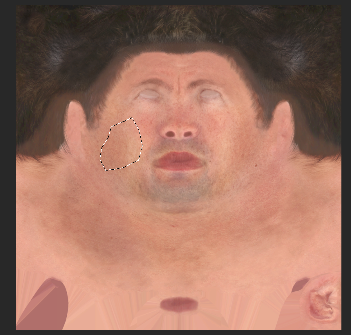
Calibrating Skin Textures During the process of making this tutorial, it has become clear that if you plan on using this technique in full production, you may wish to calibrate your skin textures. Having looked at several sets of skin textures, its clear that black skin textures tend to have more noise and blemish detail that white skin. I suspect this is to add some visual detail to skin that is difficult to bring contrast to (as its darker, there are less available color and light values). Either way, converting black skin to be lighter results in more noisey albedo textures than making lighter textures darker – which, conversely seem to lack detail. As such, its probably best to author skin at a relative mid-tone, so when blemishes, freckles, moles, scars etc. are all added, the texture is calibrated well for darker and lighter tones. You will also need to consider using a standardized base skin color on all your characters skin. If you use the same base chromophore value in all your albedo textures, then you can use the same, hard-coded shader value for all characters. In addition to all of this, I have found that, as with the noise, specular reflectance is also commonly an issue. Lighter skin, when darkened, is always significantly more ‘shiny’ than you would expect. Interestingly, dark skin made lighter does not suffer from this problem. Again, I suspect this is because white skin reflects more light generally across its surface, so issues with specular reflectance are not as noticeable. With black skin, bright highlights are instantly more noticeable. As a result I would suggest always calibrating roughness and specular textures on darker skin, and at the very least, testing across a range of skin colors. Going Further Hopefully you’re now clearer on all the topics covered in this tutorial. Its worth trying some other LUTs if you’re feeling like challenging yourself, one may be looking at Chlorophyll A & B, as see here: Some other things you could try is our shader chromophore replacement technique on other things, such as environmental assets or clothing. It should allow you to re-color just about anything, not just skin. References I used many papers and online websites over the course of this, these are the papers referenced & the papers I referred to the most: Monte Carlo Modeling of Light Transport in Tissue (Steady State and Time of Flight) Steven L. Jacques A Spectral BSSRDF for Shading Human Skin Craig Donner and Henrik Wann Jensen A Practical Appearance Model for Dynamic Facial Color Jimenez et al. A Layered, Heterogeneous Reflectance Model for Acquiring and Rendering Human Skin Donner et al Complete Project Files All the final project files are here:
Part 5: Extending the Shader
NSFW warning for further down this page Let’s take our shader and add in some new features: melanin and hemoglobin masks. Using these masks will enable us to: Melanin Masks Melanin masks are the most straightforward. We need a greyscale mask that defines area of darker skin, and areas of lighter skin. We then sample a second set of fracitonal and blend values – so we have a skin colour for lighter areas and a skin colour for darker areas. We first need to define what we’re masking We could have a single mask for all tan types, i.e. you either have a mask for natural pigmentation (palms, soles of feet) or your mask contains areas for tan lines. It is unlikely you want both, as a higher natural melanin fraction lends itself less to tan lines. For the purposes of this tutorial, we’ll use a single mask for some tan lines, but you can expand this further if you want. We’ll therefore need a one-channel mask – one for natural pigmentation and one for tan lines. I have prepared some content for you here: Direct Download: <todo: retrieve link… lost in a wordpress upgrade> Import it into our Digital Human project. In here, find open up the level Female_Tan. You will find some materials already set up with our pigmentation work from earlier. In the content I have provided, you will also see a few materials, and the following mask for tan lines: Open up the M_Female_Tan material. This is our Master Material that the different body sections inherit from, so changes here propagate to all the skin parts. It should look like this: Duplicate the recolor section in the Albedo area, double up the Input variables and rename the input scalar parameters as follows: Next, drop in our a Texture Variable, use the T_Black_Linear texture here as most body parts don’t need a texture here, and this is our default. Take the R (red) channel and drag this into a lerp node as input Alpha. We’ll set the Tan values to be input A (as tanned areas are black on our mask) and the base values to be Input B (as these are white): Now test your results on M_Female_Tan_Body by assigning our T_Melanin_Mask into the appropriate texture input: Hemoglobin Masks I wanted to use UE4 for this page, to keep things consistent. Unfortunately, I’ve been unable to source assets I can share that are high-quality, contain an ability to create facial expressions easily and are free. This is currently a one-person outfit and I don’t have the resources to make such assets in a reasonable time frame. This principles in UE4 remain the same, however. As such, of this part, we’ll be using the Digital Human Asset from the Unity Asset Store and Unity 2019.3+. Apologies for the switch, but it is necessary here (for my sanity) and never hurts to learn multiple engines for new techniques! You can get it here:<todo: again, need to get these links back> For this, we want to generate some masks that are associated with different emotions or expressions. The digital human pack provided by Unity allows for a variety of facial expressions. Unfortunately, its implementation is rather obtuse for our needs, so directly driving hemoglobin levels, while possible, will add pages to this already lengthy tutorial. Instead, we’ll use sliders to drive a couple of hemoglobin masks to demonstrate how we can use them. I have already got our basic implementation from the previous page included. Grab these files and add them to the Digital Human project mentioned above: Direct Download: To start off, you can find this texture in the assets I have provided: The red and green channels contain slightly different hemoglobin masks for the face. The first step is to add these varibales to the DigitalHuman_Skin_LUT shader graph: Then add this logic the Hemoglobin Fraction value: Compile, then make sure you add the Hemoglobin Mask to the Gawain_Skin material. Select a pale skin tone and overdo the hemoglobin to see it: Now, you can play with the expressions to get some more results: You can grab both projects, in their entirety, here:<todo: come back and fix>
Part 4: Skin Shader
Now we need to bring out LUT into a skin shader. For this tutorial, we’ll be using the Bust_Outdoors level from the Digital Human content pack, which you get through the Epic Games Launcher (via Unreal Engine -> Learn). Once you’re there, we’ll move on to some quick theory: When recolouring the skin, what we want is the ability to change just the underlying skin tone. In an ideal world, we also want to be able to texture the skin in the normal workflow way – so we texture an albedo map. This makes it easier to author, and will work with existing assets you may have. But how do we do this? If we use a Hue/Saturation/Lightness adjustment to the skin, we may end up changing the colour of the lips or other scars and blemishes, too – which is not what we want. All we want to change is the chromophore contribution to the skin tone. The solution is to divide the albedo texture by the original chromophore contribution, then multiply it by the new chromorphore contribution: α= (α/ β)γWhere α is the albedo, β is the underlying chromophore contribution, and γ is the new target chromophore contirbution. By dividing, we remove the chromophore contribution from the albedo, leaving only the remaining color contribution from blemishes, lips, etc. We can then add in a new color by multiplying it in. First, we need to get the chromophore contribution in the head texture. To do this,: Next we need to import our LUT correctly. Import the PNG we output from our Monte Carlo simulation, then double click the uasset, and change its settings to the following, then save: These are required so we keep defined edges between our 3 LUT areas – using a different filter will cause blurry edges. Clamping the texture prevents large or negative values in the shader looping back around – it just makes it less prone to user-error. Next, we shall head into UE4 and create a new Material Function called MF_SkinLUT. Open it up and construct the following: What’s going on here? We have 3 areas of our LUT for different melanin blends. We need to sample two of these areas and blend between them. For example, if we had a blend value of 0.25, we need to sample a pixel from the first LUT area (0.01 blend) and one from the second LUT area (0.5 blend), and then pick a value that is halfway between those sampled colors. We will select which pixel we sample based on melanin fraction (our “x-axis” in each area, and hemoglobin fraction is our “y-axis”) Now open up the M_Skin_Bust from the character in our scene, it contains the head skin material in this scene: Now, drag in you MF_SkinLUT material function. Add in three scalar inputs, like so: Apply the following settings to them: Next, create a Vector Parameter and set the sRGB Hex value we extracted from Photoshop: Now, divide the Albedo RGB node by this amount, then multiply that output by the output of your Material Function, just like this: Now, create a Material Instance of this Material and apply it back to your head. We do this so we can change out skin chromophore values without having to recompile shaders. You should end up with the following: Now we can start changing the skin tones! As an extension task, you can completely remove the Material Function and just multiply in any colour you like for some fantasy-genre skin tones: As you can see, we maintain pinkness in the lips (that is more evident in lighter tones) Appendix: Unity If you’re using Unity, you can use the following Shader Graph setup: The process is identical – clamp the LUT, nearest pixel filter. Here it in on the Digital Human from The Heretic project which you can grab from the Asset Store in Unity:
Part 3b (Practical): Python Imaging Library (Pillow)
We now need to write out our sRGB values to an image. We installed Pillow in the introduction, so import that now. Below our sRGB conversion loop in the Generate() function If you now run the code you should get this PNG output – its small, so I’ve zoomed in: We obviously want more fidelity. We have two options: increase the samples (which is an exponential performance cost), or just use Photoshop to resize it. We’ll do the latter as its much faster, as gives us enough gradation. To do this, we need to select each 1/3 of the LUT, which is each melanin blend and resize it using a “bicubic smoother” filter to smooth the gradations out, like so: 1. Select the first 1/3: 2. Copy it to a new image and resize 3. Repeat for the other two LUT sections, then composite them into a new 192*46 pixel image Great! You have got yourself a look-up texture based on physical spectral absorption values! For reference, here’s the complete project so far: Next we’ll be getting this into Unreal Engine 4.
Part 3 (Practical): Spectral Reflection & Color Spaces
XYZ Spectral Sensitivity Curves First, let’s get those Gaussian curves for the XYZ spectral sensitivity curves. I’ve pre-generated these into (you guessed it, CSV). Put this into your development directory, with everything else: In our __init__ function, do the following: And declare at the top of our class, CIE_CMF: CIE_XYZ_Spectral_Sensitivity_Curve = {} This will store the values in a dictionary. RGB Matrices Now to add in our RGB matrix and gamma correction for sRGB: Converting Our Data Our data isn’t in a usable state yet. We need to restructure the data coming from the Monte Carlo simulation to be organised by melanin blend, melanin fraction, hemoglobin fraction – this is so we can output a pixel of colour for each value. We’ll replace all our CSV output code, and instead of returning a string, we’ll return tuples of the values, like so: And adjust the generate function: Now, above the return statement add the following to convert all our data to sRGB: Next step, we’ll make an image! For reference, current code:
Part 3 (Theory): Spectral Reflection & Color Spaces
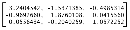
Having spectral reflectance values is all well-and-good, but this still isn’t a color we can use in a look-up table. Representing Spectral Reflection Values How do we go about converting this data into something usable? Fortunately much of this work has already been done by the Commission internationale de l’éclairage (‘CIE’, pronounced ‘see’). Human sight is broadly defined as being receptive to 3 colors: red, green and blue. This isn’t strictly true, as discussed previously, these categorizations are human constructs and don’t accurately reflect what is actually happening. The human eye has 3 cones receptive to 3 different spectrums of visible light. Here they are illustrated across the visible spectrum: We could multiply our reflectance values by these stimulus curves to get three color values. However, due to the distribution of cones in the human eye, the values to multiply by are actually dependent on the observer’s field of view. Captain Dissilusion has a great little primer on color here, and is worth a watch: The CIE Standard Observer and XYZ Color Space To solve this problem, CIE has defined a color-mapping function we can use that standardizes on the 2º FOV. It looks like this: If we multiply our reflectance values by each of these color-matching functions, we will given three values, X, Y and Z. These are not RGB values. RGB is a color space – a way of numerically storing colours. XYZ is another type of color space. The CIE XYZ is a device-invariant way of storing color and we use it because not all colors are equal – is is possible to have two colors that are the same, but are composed of different wavelengths of light. CIE XYZ is also a space from which you can convert to any other color space, such as RGB, sRGB, HSV, etc. We can generate these curves using Gaussian functions. Gaussian functions are used to create parabola-like curves. We can generate them the following way: By multiplying our reflectance values by this, we can obtain CIE XYZ values. The sRGB Color Space Now to convert them to usable color information for textures. We’ll convert them to sRGB as this is what we’ll need to textures in UE4. To do this, we multiply our XYZ values by the RGB matrix for the 2º observer, with the D65 illuminant. r = x * m[0][0] + y * m[0][1] + z * m[0][2]g = x * m[1][0] + y * m[1][1] + z * m[1][2]b = x * m[2][0] + y * m[2][1] + z * m[2][2] In order to now get this into sRGB, we simply do a gamma correction: if abs(c) > 0.0031308 c = 1.055 * c1/2.2 -0.055else c = 12.92 * cwhere c is one of our channels, r, g or b After all of that work, we now have sRGB colours from our reflectance values. Now, we’ll implement it
Part 2 (Practical): The Monte Carlo Simulation
We’ll take what we learned in the previous part and start fleshing out our Monte Carlo (“MC”) simulation. First, let’s import the random and math classes – we’ll need them. In our Python script, we’ll add a new function to our class. We’ll call this MonteCarlo. As its inputs, we need these parameters from our spectral work: σepidermisa, σepidermiss, σdermisa, σdermiss and λ We’ll need two more utility functions. One is the Fresnel function, the second is a quick sign(x) function. Add these to the class, too: The next step is to add the following values to our Monte Carlo function. These are values we need for our light transport: Lets now create all the variables we need to change, such as position, trajectory, bins, weight, etc.: And the last thing before we begin looping; some initialization: Now we can begin our iteration code. We’ll start with a simple while loop for number of photons: Within this loop, we need to do some further initialization for this loop: W = 1.0photon_status = ALIVE x= 0y = 0z = 0 #Randomly set photon trajectory to yield an isotropic source.costheta = 2.0 * random.random() – 1.0 sintheta = math.sqrt(1.0 – costheta*costheta)psi = 2.0 * PI * random.random()ux = sintheta * math.cos(psi)uy = sintheta * math.sin(psi)uz = (abs(costheta)) # on the first step we want to head down, into the tissue, so > 0 # Propagate one photon until it dies as determined by ROULETTE.# or if it reaches the surface againit = 0max_iterations = 100000 # to help avoid infinite loops in case we do something wrong # we’ll hit epidermis first, so set mua/mus to those scattering/absorption valuesmua = epi_muamus = epi_musalbedo = epi_albedo W = 1.0 photon_status = ALIVE x= 0 y = 0 z = 0 #Randomly set photon trajectory to yield an isotropic source. costheta = 2.0 * random.random() – 1.0 sintheta = math.sqrt(1.0 – costheta*costheta) psi = 2.0 * PI * random.random() ux = sintheta * math.cos(psi) uy = sintheta * math.sin(psi) uz = (abs(costheta)) # on the first step we want to head down, into the tissue, so > 0 # Propagate one photon until it dies as determined by ROULETTE. # or if it reaches the surface again it = 0 max_iterations = 100000 # to help avoid infinite loops in case we do something wrong # we’ll hit epidermis first, so set mua/mus to those scattering/absorption values mua = epi_mua mus = epi_mus albedo = epi_albedo W = 1.0 photon_status = ALIVE W = 1.0 photon_status = ALIVE x= 0 y = 0 z = 0 #Randomly set photon trajectory to yield an isotropic source. costheta = 2.0 * random.random() – 1.0 sintheta = math.sqrt(1.0 – costheta*costheta) psi = 2.0 * PI * random.random() ux = sintheta * math.cos(psi) uy = sintheta * math.sin(psi) uz = (abs(costheta)) # on the first step we want to head down, into the tissue, so > 0 # Propagate one photon until it dies as determined by ROULETTE. # or if it reaches the surface again it = 0 max_iterations = 100000 # to help avoid infinite loops in case we do something wrong # we’ll hit epidermis first, so set mua/mus to those scattering/absorption values mua = epi_mua mus = epi_mus albedo = epi_albedo This will so far spawn a photon and do nothing. We now need to implement that flow chart from the Theory part; launch, hop, drop, spin, terminate. Let’s make a new loop within the existing one. The first thing we have to do is add a break condition – for now, we’ll put in a max iteration, but we’ll also add in our terminate functionality. while True: it = it + 1 # Check Roulette if (W < THRESHOLD): if (random.random() <= CHANCE): W = W / CHANCE else: photon_status = DEAD if photon_status is DEAD: break if it > max_iterations: break while True: it = it + 1 # Check Roulette if (W < THRESHOLD): if (random.random() <= CHANCE): W = W / CHANCE else: photon_status = DEAD if photon_status is DEAD: break if it > max_iterations: break while True: it = it + 1 # Check Roulette if (W < THRESHOLD): if (random.random() <= CHANCE): W = W / CHANCE else: photon_status = DEAD if photon_status is DEAD: break if it > max_iterations: break Above the ‘# Check Roulette‘ line, we’ll flesh out our hop code: # Check Roulette # Check Roulette # Check Roulette rnd = random.random() while rnd <= 0.0: # make sure it is > 0.0 rnd = random.random() s = -math.log(rnd)/(mua + mus) x = x + (s * ux) y = y + (s * uy) z = z + (s * uz) rnd = random.random() while rnd <= 0.0: # make sure it is > 0.0 rnd = random.random() s = -math.log(rnd)/(mua + mus) x = x + (s * ux) y = y + (s * uy) z = z + (s * uz) rnd = random.random() while rnd <= 0.0: # make sure it is > 0.0 rnd = random.random() s = -math.log(rnd)/(mua + mus) x = x + (s * ux) y = y + (s * uy) z = z + (s * uz) On our first ‘hop’, the code is the ‘launch’ step. Immediately after this, we do a boundary check to see if the photon is escaping the skin, moving back to the boundary as needed: if uz < 0: # calculate partial step to reach boundary surface s1 = abs(z/uz) # move back x = x – (s * ux) y = y – (s * uy) z = z – (s * uz) # take partial step x = x + (s1 * ux) y = y + (s1 * uy) z = z + (s1 * uz) if uz < 0: # calculate partial step to reach boundary surface s1 = abs(z/uz) # move back x = x – (s * ux) y = y
Part 2 (Theory): The Monte Carlo Simulation
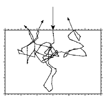
Introduction As discussed in previous chapters, we need to simulate light photon beams in order to determine the true color of our surface. The “Monte Carlo” simulation provides a method to do this. The name “Monte Carlo” derives from the randomness used in the method; we use random values at several stages and also use a Russian Roulette approach to ‘killing’ the photon beam. The general approach is to create a beam of light at a position (i.e. the origin, (0,0,0)), give it a direction and wavelength. We then iterate for n times, each time moving the photon beam further into the material, scattering, absorbing and reflecting as it goes. We run the simulation for each wavelength of light we care about – i.e. 380nm-780nm, at 10nm intervals. We store the information we want to keep (in our case, the reflectance) in “bins” that we add to at each iteration stage. Here’s the general flow for Monte Carlo simulation: To translate this: We launch a photon with a weight (w = 1.0), we move the photon (hop) and check if we have changed boundaries between tissues. At the drop stage we interact with the tissue (absorption, etc). Next, we redirect the photon based on scattering (spin), and finally we run a simple roulette to see if the photon should terminate. If we don’t terminate, we keep moving the photon. If it does terminate, we launch the next photon. This process continues until we run out of photons (N photons). We will now cover each of these steps more deeply: Launch To launch we need three things:1. A starting location2. A starting direction to hop3. A “weight” The first two should be fairly explanatory. We start at (0,0,0) and initially move forwards – we will use +z as our forward axis into the tissue. We will use an “isotropic point source” to launch our photon. This simply means we have no preferred direction. Our starting position shall be: x = 0, y = 0, z = 0 And our launching trajectory will be: RND = 0.0 <= n < 1.0cosθ = 2 RND – 1 sinθ = √(1-cosθ)ϕ = 2 π RNDif ( ϕ < π ) sinϕ = √(1-cos2ϕ)else sinϕ = –√(1-cos2ϕ) ux = sinθ cosϕuy = sinθ sinϕuz = abs(cosθ) The weight, w, is what we shall use to track how much of the photon’s energy is remaining. In our simulation we shall define a zone around the origin through which we will collect any photons that head back into it. By summing the weight of these photons, at all the wavelengths of light we are sampling, we will end up with our reflectance values. Hop Hop consists of two parts: A Boundary Check and Moving. In our two-layer model, we have an upper epidermis, a lower dermis layer and the external medium – air. For our purposes, we count anything above the epidermis as ‘escaped’, and if it is close enough to the beam source (the launch position), we capture its weight. We’ll start by calculating our new position, this is calculated by: µt = µa + µswhere µa is the absorption coefficient, and µs is our scattering coefficient s = -ln(RND)/µtx = x + s uxy = y + s uyz = z + s uz Now we check whether it has escaped the tissue by checking if the uz property is < 0.0. However, the photon may partially reflect back into the tissue at the boundary, due to total internal reflection. How do we calculate this? First, let’s start by moving the photon back to the point where it left the tissue, and move it just back to the surface. We calculate the partial step, s1: s1 = abs(z/uz) Then, retract the full step: x = x – s uxy = y – s uyz = z – s uz and then add in the partial step, back to the boundary: x = x + s1 uxy = y + s1 uyz = z + s1 uz Now our photon is at the surface, we use the Fresnel equation to determine how much of the energy was reflected back into the tissue: We can now calculate the weight that has escaped the tissue with: Re = 1 – Ri This can then be stored in our ‘bin’ r = √(x2 + y2)ir = r/drreflectionBin[ir] = Re where dr is our radial bin size, (radial size of our photons/number of bins). I have glossed over these parameters, as its a bit deep for this tutorial. Simply put, r is the radial position of the photon, dr gives us a ‘depth’. Although we simulate the Monte Carlo simulation in 3D Cartesian coordinates, we actually only care about getting data for radial position and depth, as the photon beam is cylindrical. Finally, we bounce the photon back into the tissue, with it’s escapes weighting removed: w = Ri * wuz = -uzx = (s-s1) * uxy = (s-s1) * uyz = (s-s1) * uz Drop Our drop stage is the easiest. As we have calculated the reflectance of the tissue above, we simply need to decrement the weight of our photon by the amount absorbed by the surface albedo. Which albedo value we use depends on the layer in the skin we are in: if z <= epidermis_thickness albedo = σepidermiss/(σepidermiss + σepidermisa)else albedo = σdermiss/(σdermiss + σdermisa) Now to reduce the weight: absorb = w * (1 – albedo)w = w – absorb Spin Next up: scatter the photon! We need two angles of scatter, θ (deflection) and ϕ (azimuthal). The source paper goes into great detail as to why we use the following formula (the HG function) to calculate θ, if you want more information, but for the purposes of this tutorial, we’ll just describe it: The azimuthal angle is a bit less verbose: ϕ = 2π RND Now we can calculate the new angles, we need to update our photon trajectories: if (1 – abs(uz) <= 1 – cos0)